User’s guide
Business dates
Business dates handling capabilities is provided by the quantlib.time subpackage. The three core components are Date, Period and Calendar.
Date
A date in QuantLib can be constructed with the following syntax:
Date(serial_number)
where serial_number is the number of days such as 24214, and 0 corresponds to 31.12.1899. This date handling is also known from Excel. The alternative is the construction via:
Date(day, month, year)
Here, day, month and year are of integer. A set of month constant are available in the date module (January, …, December or Jan, …, Dec)
After constructing a Date, we can do simple date arithmetics, such as adding/subtracting days and months to the current date. Furthermore, the known convenient operators such as +=,-= can be used.
It is possible to add a Period to a date. Period can be created using time units or frequency:
Period(frequency)
Period(lenght, time_units)
Frequencies are defined with the following constants: NoFrequency, Once, Annual, Semiannual, EveryFourthMonth, Quartely, Bimonthly, Monthly, EveryFourthWeek, Biweekly, Weekly, Daily and OtherFrequency.
Time units are constants defined in the date module: Days, Weeks, Months, Years.
Each Date object has the following properties:
weekdayreturns the weekday using the weekday constants defined in the date module (Sunday to Saturday and Sun to Sat).dayreturns the day of the monthday_of_yearreturns the day of the yearmonthreturns the monthyearreturns the yearserialreturns a the serial number of this date
The quantlib.time.date module has some useful static functions,
which give general results, such as whether a given year is a leap
year or a given date is the end of the month. The currently available
functions are:
today()mindate(): earliest possible Date in QuantLibmaxdate(): latest possible Date in QuantLibis_leap(): is year a leap year?end_of_month(): what is the end of the current month the date is in?is_end_of_month(date)(): is date the end of the month?next_weekday(date, weekday)(): on which date is the weekday following the date? (e.g. date of the next Friday)nth_weekday(n, weekday, month, year)(): what is the n-th weekday in the given year and month? (e.g. date of the 3rd Wednesday in July 2010)
Calendars
One of the crucial objects in the daily business is a calendar for different countries which shows the holidays, business days and weekends for the respective country. In QuantLib, a calendar can be set up easily via:
uk_calendar = UnitedKingdom()
for the UK. Calendars implementation are available in the
quantlib.time.calendars subpackage.
Various other calendars are available, for example for Germany, United States, Switzerland, Ukraine, Turkey, Japan, India, Canada and Australia. In addition, special exchange calendars can be initialized for several countries. For example, the New-York Stock Exchange calendar can be initialized via:
us_calendar = UnitedStates(NYSE);
The following functions are available:
is_business_day(date)()is_holiday(date)()is_weekend(week_day)(): is the given weekday part of the weekend?is_end_of_month(date)(): indicates, whether the given date is the last business day in the month.end_of_month(date)(): returns the last business day in the month.
The calendars are customizable, so you can add and remove holidays in your calendar:
addHoliday(date)()removeHoliday(date)(): removes a user specified holiday
Furthermore, a function is provided to return a list of holidays
holidayList(calendar, from_date, to_date, include_weekends=False)(): returns a holiday list, including or excluding weekends. This function returns a DateList object that provides an list/iterator-like interface on top of the C++ QuantLib date vector.
Adjusting a date can be necessary, whenever a transaction date falls on a date that is not a business day.
The following Business Day Conventions are available in the calendar module:
- Following: the transaction date will be the first following day that is a business day.
- ModifiedFollowing: the transaction date will be the first following day that is a business day unless it is in the next month. In this case it will be the first preceding day that is a business day.
- Preceding: the transaction date will be the first preceding day that is a business day.
- ModifiedPreceding: the transaction date will be the first preceding day that is a business day, unless it is in the previous month. In this case it will be the first following day that is a business day.
- Unadjusted
- The Calendar functions which perform the business day adjustments are :
- adjust(date, business_day_convention)
- advance(date,period, business_day_convention, end_of_month): the end_of_month variable enforces the advanced date to be the end of the month if the current date is the end of the month.
Finally, it is possible to count the business days between two dates with the following function:
- business_days_between(from_date, to_date, include_first, include_last) calculates the business days between from and to including or excluding the initial/final dates.
We will demonstrate an example by using the Frankfurt Stock Exchange calendar and the dates Date(31,Oct,2009) and Date(1,Jan,2010). From the first date, we advance 2 months in the future, which is December, 31st. Since this is a holiday and the next business day is in the next month, we can check the Modified Following conversion. The Modified Preceding conversion can be checked for January, 1st 2010:
frankfcal   = Germany(FrankfurtStockExchange);
first_date  = Date(31,Oct,2009)
second_date = Date(1,Jan ,2010);

print "Date 2       Adv:", frankfcal.adjust(second_date , Preceding)
print "Date 2       Adv:", frankfcal.adjust(second_date , ModifiedPreceding)

mat = Period(2,Months)

print "Date 1 Month Adv:", \
  frankfcal.avance(
        first_date, period=mat, convention=Following,
        end_of_month=False
   )
print "Date 1 Month Adv:", \
  frankfcal.avance(
        first_date, period=mat, convention=ModifiedFollowing,
        end_of_month=False
  )
print "Business Days Between:", \
  frankfcal.business_days_between(
        first_date, second_date, False, False
  )
and the output will give
Date 2       Adv: 30/12/2009
Date 2       Adv:  4/01/2010
Date 1 Month Adv:  4/01/2010
Date 1 Month Adv: 30/12/2009
Business Days Between: 41
Day counters
Daycount conventions are crucial in financial markets. QuantLib offers :
- Actual360: Actual/360 day count convention
- Actual365Fixed: Actual/365 (Fixed)
- ActualActual: Actual/Actual day count
- Business252: Business/252 day count convention
- Thirty360: 30/360 day count convention
The construction is easily performed via:
myCounter = ActualActual()
The other conventions can be constructed equivalently. The available functions are :
- dayCount(from_date, to_date)
- yearFraction(from_date, to_date)
TODO : add example
Date generation
An often needed functionality is a schedule of payments, for example for coupon payments of a bond. The task is to produce a series of dates from a start to an end date following a given frequency(e.g. annual, quarterly…). We might want the dates to follow a certain business day convention. And we might want the schedule to go backwards (e.g. start the frequency going backwards from the last date).
For example:
- Today is Date(3,Sep,2009). We need a monthly schedule which ends at Date(15,Dec,2009). Going forwards would produce Date(3,Sep,2009),Date(3,Oct,2009),Date(3,Nov,2009),Date(3,Dec,2009) and the final date Date(15,Dec,2009).
- Going backwards, on a monthly basis, would produce Date(3,Sep,2009),Date(15,Sep,2009),Date(15,Oct,2009), Date(15,Nov,2009),Date(15,Dec,2009).
The different procedures are given by the DateGeneration object and will now be summarized:
- Backward: Backward from termination date to effective date.
- Forward: Forward from effective date to termination date.
- Zero: No intermediate dates between effective date and termination date.
- ThirdWednesday: All dates but effective date and termination date are taken to be on the third Wednesday of their month (with forward calculation).
- Twentieth: All dates but the effective date are taken to be the twentieth of their month (used for CDS schedules in emerging markets). The termination date is also modified.
- TwentiethIMM: All dates but the effective date are taken to be the twentieth of an IMM month (used for CDS schedules). The termination date is also modified.
The schedule is initialized by the Schedule class:
Schedule(effective_date , termination_date, tenor, calendar, convention ,
         termination_date_convention , date_gen_rule,
         end_of_month, first_date, next_to_last_date)
The arguments represent the following
- effective_date, termination_date: start/end of the schedule
- tenor: a Period object reprensenting the frequency of the schedule (e.g. every 3 months)
- termination_date_convention: allows to specify a special business day convention for the final date.
- rule: the generation rule, as previously discussed
- end_of_month: if the effective date is the end of month, enforce the schedule dates to be end of the month too (termination date excluded).
- first_date, next_to_last_date: are optional parameters. If we generate the schedule forwards, the schedule procedure will start from first_date and then increase in the given periods from there. If next_to_last_date is set and we go backwards, the dates will be calculated relative to this date.
The Schedule object has various useful functions, we will discuss some of them.
- size(): returns the number of dates
- at(i) : returns the date at index i.
- previous_date(ref_date): returns the previous date in the schedule compared to a reference date.
- next_date(ref_date): returns the next date in the schedule compared to a reference date.
- dates(): returns the whole schedule in a DateList object.
Performance considerations
In [3]: %timeit QuantLib.Date.todaysDate() + QuantLib.Period(10, QuantLib.Days) 100000 loops, best of 3: 9.71 us per loop
In [4]: %timeit datetime.date.today() + datetime.timedelta(days=10) 100000 loops, best of 3: 3.55 us per loop
In [5]: %timeit quantlib.date.today() + quantlib.date.Period(10, quantlib.date.Days) 100000 loops, best of 3: 2.17 us per loop
Reference
The mlab module provides high-level functions suitable for easily performing common quantitative finance calculations. These functions use as input standardized data structures that are provided to limit the amount of data transformation needed to string functions together.
The mlab functions often use pandas data frames as inputs. In order to encourage inter-operability between functions, we have defined a number of standard data structures. The column names of these data frames are defined in the ‘’names’’ module. The standardized data structures should be created with the functions provided in the ‘’data_structures’’ module.
Names
The column names of all datasets are defined in names.py. A column name should always be referenced by the corresponding variable name, and not by a character string. For example, refer to the ‘Strike’ column of an option_quotes data set by:
import quantlib.reference.names as nm
strike = option_quotes[nm.STRIKE]
rather than:
strike = option_quotes['Strike']
Data Structures Templates
These data structures are defined to facilitate the inter-operability of the high level functions found in the ‘mlab’ module.
Option Quotes
This data structure contains the necessary data for calibrating a stochastic model for the underlying asset, also known as volatility model.
An option quotes data structure with 10 rows is created with the statements:
import quantlib.reference.data_structures as ds
option_quotes = ds.option_quotes_template().reindex(index=range(10))
Risk-free Rate and Dividends
When calibrating a volatility model, the default algorithm is to compute the implied term structure of risk-free rate and dividend yield from the option data, using the call-put parity relationship. The result of this calculation is the ‘riskfree_dividend’ data structure.
Mlab
The mlab module provides high-level functions suitable for easily performing common quantitative finance calculations. These functions use as input standardized data structures that are provided to limit the amount of data transformation needed to string functions together.
Standardized data structures
Curve building
Asset pricing
Notebooks
The notebooks and scripts folder provide sample calculations performed with QuantLib.
Getting started
In order to use the notebokks, you need to install:
- Ipython 0.13
- pylab
- matplotlib
Make sure that pyQL is in the PYTHONPATH. You can access the notebooks with the command:
ipython notebook --pylab inline <path to the notebooks folder> --browser=<browser name>
For example, on a linux system where the pyql project is located in ~/dev, the command to view the notebooks with the Firefox browser would be:
ipython notebook --pylab inline ~/dev/pyql/examples/notebooks --browser=firefox
The browser will start and display a menu with several notebooks. As of October 2012, you should see 8 notebooks, as shown below:
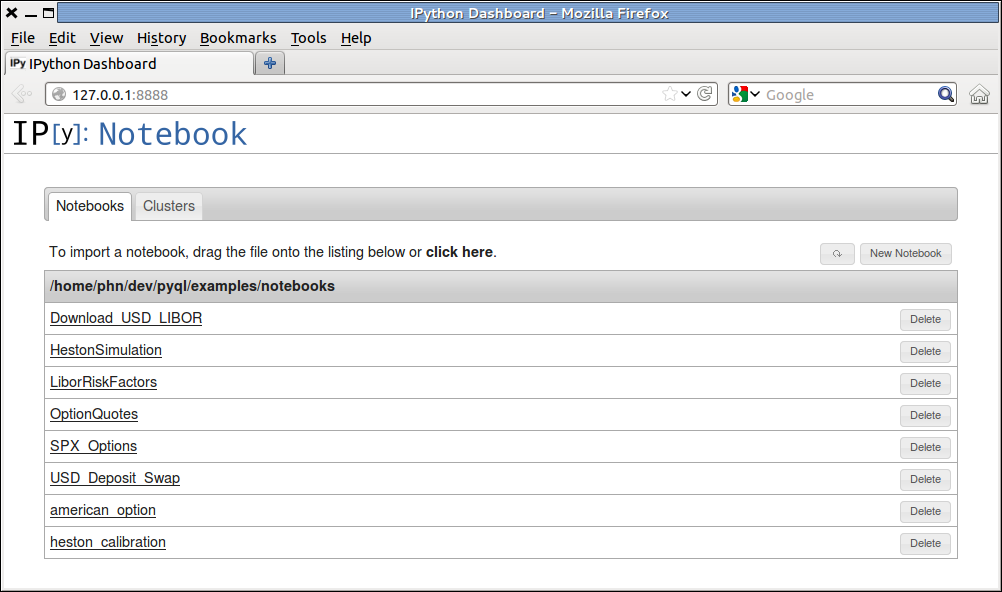
Notebook menu in the Firefox browser.